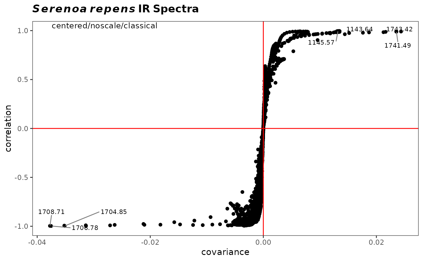
Produces a scatter plot of the correlation of the variables against their covariance for a chosen principal component. It allows visual identification of variables driving the separation and thus is a useful adjunct to traditional loading plots.
sPlotSpectra(spectra, pca, pc = 1, tol = 0.05, ...)Arguments
- spectra
An object of S3 class
Spectra().- pca
The result of a pca calculation on
Spectra(i.e. the output fromc_pcaSpectraorr_pcaSpectra).- pc
An integer specifying the desired pc plot.
- tol
A number describing the fraction of points to be labeled.
tol = 1.0labels all the points;tol = 0.05labels approximately the most extreme 5 percent. Set to'none'to completely suppress labels. Note that a simple approach based upon quantiles is used, assumes that both x and y are each normally distributed, and treats x and y separately. Thus, this is not a formal treatment of outliers, just a means of labeling points. Groups are lumped together for the computation.- ...
Parameters to be passed to the plotting routines. Applies to base graphics only.
Value
The returned value depends on the graphics option selected (see ChemoSpecUtils::GraphicsOptions()).
base: None. Side effect is a plot.ggplot2: The plot is displayed, and aggplot2object is returned if the value is assigned. The plot can be modified in the usualggplot2manner.
References
Wiklund, Johansson, Sjostrom, Mellerowicz, Edlund, Shockcor, Gottfries, Moritz, and Trygg. "Visualization of GC/TOF-MS-Based Metabololomics Data for Identification of Biochemically Interesting Compounds Usings OPLS Class Models" Analytical Chemistry Vol.80 no.1 pgs. 115-122 (2008).
See also
Additional documentation at https://bryanhanson.github.io/ChemoSpec/
Examples
# This example assumes the graphics output is set to ggplot2 (see ?GraphicsOptions).
library("ggplot2")
data(SrE.IR)
pca <- c_pcaSpectra(SrE.IR)
myt <- expression(bolditalic(Serenoa) ~ bolditalic(repens) ~ bold(IR ~ Spectra))
p <- sPlotSpectra(spectra = SrE.IR, pca = pca, pc = 1, tol = 0.001)
p <- p + ggtitle(myt)
p
