Plot PCA Loadings from a Spectra Object Against Each Other
Source:R/plot2Loadings.R
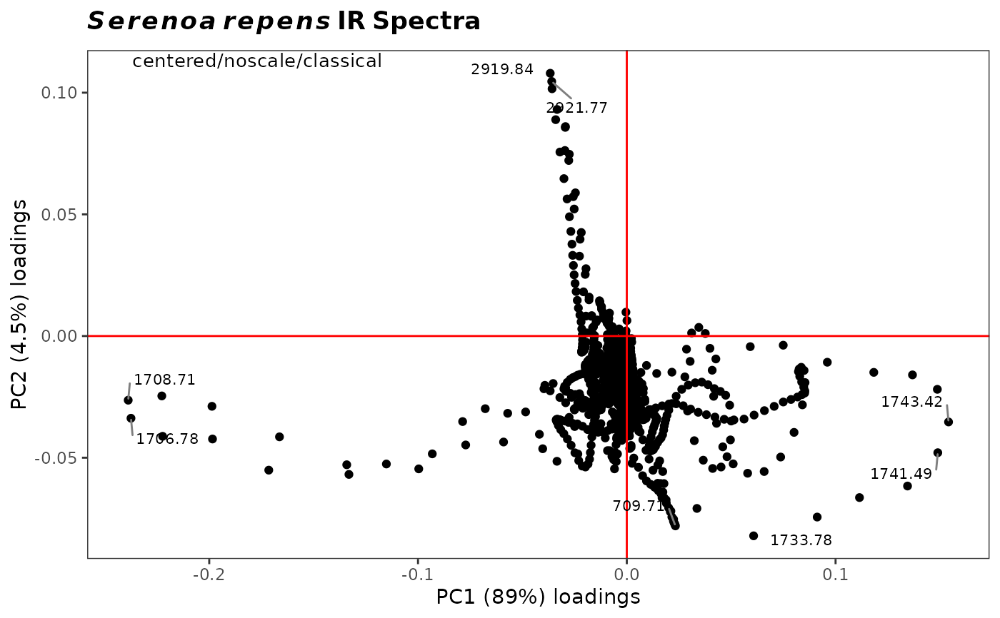
plot2Loadings.RdPlots two PCA loadings specified by the user, and labels selected (extreme) points. Typically used to determine which variables (frequencies) are co-varying, although in spectroscopy most peaks are represented by several variables and hence there is a lot of co-varying going on. Also useful to determine which variables are contributing the most to the clustering on a score plot.
plot2Loadings(spectra, pca, loads = c(1, 2), tol = 0.05, ...)Arguments
- spectra
An object of S3 class
Spectra().- pca
An object of class
prcomp, modified to include a list element called$method, a character string describing the pre-processing carried out and the type of PCA performed (it appears on the plot). This is automatically provided ifChemoSpecfunctionsc_pcaSpectraorr_pcaSpectrawere used to createpca.- loads
A vector of two integers specifying which loading vectors to plot.
- tol
A number describing the fraction of points to be labeled.
tol = 1.0labels all the points;tol = 0.05labels approximately the most extreme 5 percent. Set to'none'to completely suppress labels. Note that a simple approach based upon quantiles is used, assumes that both x and y are each normally distributed, and treats x and y separately. Thus, this is not a formal treatment of outliers, just a means of labeling points. Groups are lumped together for the computation.- ...
Parameters to be passed to the plotting routines. Applies to base graphics only.
Value
The returned value depends on the graphics option selected (see ChemoSpecUtils::GraphicsOptions()).
base: None. Side effect is a plot.ggplot2: The plot is displayed, and aggplot2object is returned if the value is assigned. The plot can be modified in the usualggplot2manner.
See also
See plotLoadings to plot one loading against the
original variable (frequency) axis. See sPlotSpectra for
a different approach. Additional documentation at
https://bryanhanson.github.io/ChemoSpec/
Examples
# This example assumes the graphics output is set to ggplot2 (see ?GraphicsOptions).
library("ggplot2")
data(SrE.IR)
pca <- c_pcaSpectra(SrE.IR)
myt <- expression(bolditalic(Serenoa) ~ bolditalic(repens) ~ bold(IR ~ Spectra))
p <- res <- plot2Loadings(SrE.IR, pca, loads = c(1, 2), tol = 0.001)
p <- p + ggtitle(myt)
p