Remove Peaks in a Spectra2D Object

This function sets peaks at specified frequencies in a Spectra2D object to NA. This effectively removes these peaks from calculations of contours which can speed things up and clarifies the visual presentation of data. This function is useful for removing regions with large interfering peaks (e.g. the water peak in 1H NMR), or regions that are primarily noise. This function leaves the frequency axes intact. Note that the parafac function, used by pfacSpectra2D, does not allow NA in the input data matrices. See removeFreq for a way to shrink the data set without introducing NAs.

removePeaks2D(spectra, remF2 = NULL, remF1 = NULL)

Arguments

spectra	An object of S3 class Spectra2D from which to remove selected peaks.
remF2	A formula giving the range of frequencies to be set to NA. May include "low" or "high" representing the extremes of the spectra. Values outside the range of F2 are tolerated without notice and are handled min or max.See the examples.
remF1	As for remF2.

Value

An object of S3 class Spectra2D.

See also

removeFreq.

Author

Bryan A. Hanson, DePauw University.

Examples

# Note we will set contours a bit low to better
# show what is going on.

data(MUD1)

plotSpectra2D(MUD1,
  which = 7, lvls = 0.1, cols = "black",
  main = "MUD1 Sample 7: Complete Data Set"
)

MUD1a <- removePeaks2D(MUD1, remF2 = 2.5 ~ 4)
sumSpectra(MUD1a)
#> 
#>  MUD1: HSQC-like data for testing. See ?MUD1 
#> 
#> 	There are 10 spectra in this set.
#> 
#> 	The F2 dimension runs from 0 to 5 ""^1 * H ~ ppm
#> 	and there are 100 data points.
#> 
#> 	The F1 dimension runs from 10 to 80 ""^13 * C ~ ppm
#> 	and there are 50 slices.
#> 
#> 	NAs were found in the data matrices.  To see where, use plotSpectra2D.
#> 
#> 	The spectra are divided into 2 groups: 
#> 
#>     group no. color
#> 1 Alcohol   5 black
#> 2   Ether   5   red
#> 
#> *** Note: this is an S3 object
#> of class 'Spectra2D'
plotSpectra2D(MUD1a,
  which = 7, lvls = 0.1, cols = "black",
  main = "MUD1 Sample 7\nRemoved Peaks: F2 2.5 ~ 4"
)

MUD1b <- removePeaks2D(MUD1, remF2 = low ~ 2)
sumSpectra(MUD1b)
#> 
#>  MUD1: HSQC-like data for testing. See ?MUD1 
#> 
#> 	There are 10 spectra in this set.
#> 
#> 	The F2 dimension runs from 0 to 5 ""^1 * H ~ ppm
#> 	and there are 100 data points.
#> 
#> 	The F1 dimension runs from 10 to 80 ""^13 * C ~ ppm
#> 	and there are 50 slices.
#> 
#> 	NAs were found in the data matrices.  To see where, use plotSpectra2D.
#> 
#> 	The spectra are divided into 2 groups: 
#> 
#>     group no. color
#> 1 Alcohol   5 black
#> 2   Ether   5   red
#> 
#> *** Note: this is an S3 object
#> of class 'Spectra2D'
plotSpectra2D(MUD1b,
  which = 7, lvls = 0.1, cols = "black",
  main = "MUD1 Sample 7\nRemoved Peaks: F2 low ~ 2"
)

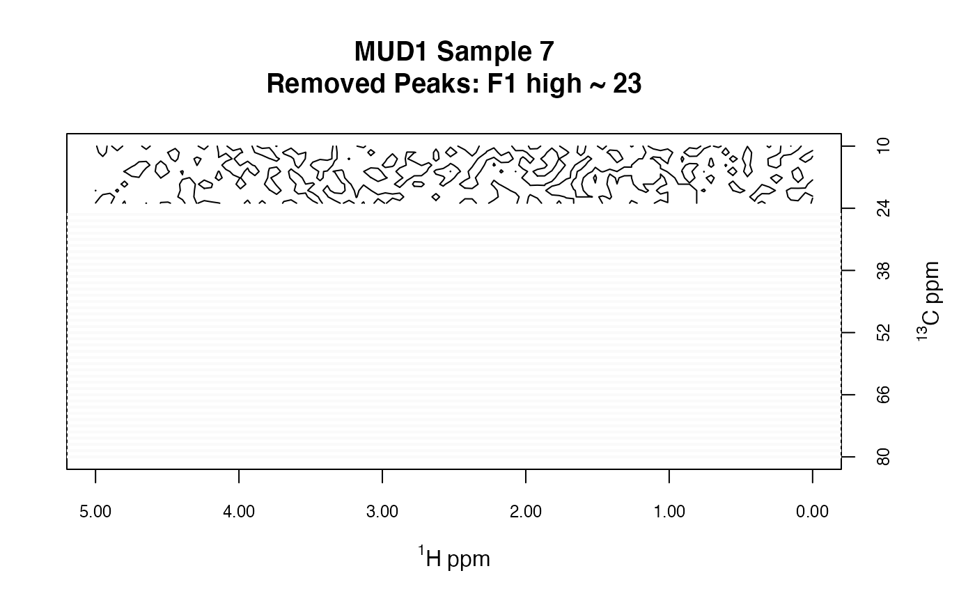
MUD1c <- removePeaks2D(MUD1, remF1 = high ~ 23)
sumSpectra(MUD1c)
#> 
#>  MUD1: HSQC-like data for testing. See ?MUD1 
#> 
#> 	There are 10 spectra in this set.
#> 
#> 	The F2 dimension runs from 0 to 5 ""^1 * H ~ ppm
#> 	and there are 100 data points.
#> 
#> 	The F1 dimension runs from 10 to 80 ""^13 * C ~ ppm
#> 	and there are 50 slices.
#> 
#> 	NAs were found in the data matrices.  To see where, use plotSpectra2D.
#> 
#> 	The spectra are divided into 2 groups: 
#> 
#>     group no. color
#> 1 Alcohol   5 black
#> 2   Ether   5   red
#> 
#> *** Note: this is an S3 object
#> of class 'Spectra2D'
plotSpectra2D(MUD1c,
  which = 7, lvls = 0.1, cols = "black",
  main = "MUD1 Sample 7\nRemoved Peaks: F1 high ~ 23"
)

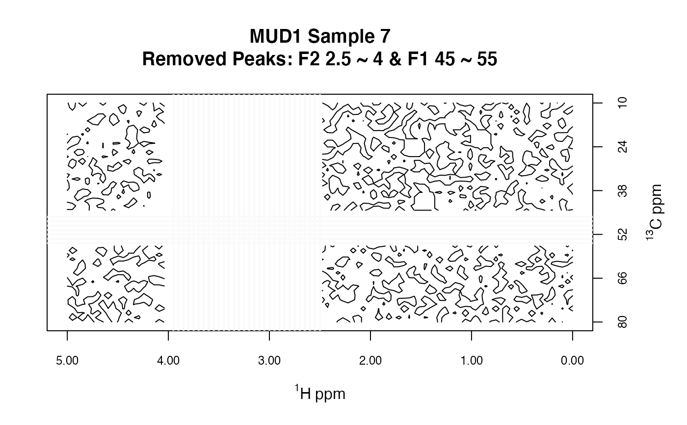
MUD1d <- removePeaks2D(MUD1, remF2 = 2.5 ~ 4, remF1 = 45 ~ 55)
sumSpectra(MUD1d)
#> 
#>  MUD1: HSQC-like data for testing. See ?MUD1 
#> 
#> 	There are 10 spectra in this set.
#> 
#> 	The F2 dimension runs from 0 to 5 ""^1 * H ~ ppm
#> 	and there are 100 data points.
#> 
#> 	The F1 dimension runs from 10 to 80 ""^13 * C ~ ppm
#> 	and there are 50 slices.
#> 
#> 	NAs were found in the data matrices.  To see where, use plotSpectra2D.
#> 
#> 	The spectra are divided into 2 groups: 
#> 
#>     group no. color
#> 1 Alcohol   5 black
#> 2   Ether   5   red
#> 
#> *** Note: this is an S3 object
#> of class 'Spectra2D'
plotSpectra2D(MUD1d,
  which = 7, lvls = 0.1, cols = "black",
  main = "MUD1 Sample 7\nRemoved Peaks: F2 2.5 ~ 4 & F1 45 ~ 55"
)