PARAFAC Analysis of a Spectra2D Object

Carry out PARAFAC analysis of a Spectra2D object. Function parafac from multiway is used. For large data sets, computational time may be long enough that it might desirable to run in batch mode and possibly use parallel processing.

pfacSpectra2D(spectra, parallel = FALSE, setup = FALSE, nfac = 2, ...)

Arguments

spectra: An object of S3 class Spectra2D.
parallel: Logical. Should parallel processing be used? Unless you love waiting, you should use parallel processing for larger data sets. If you are working on a shared machine and/or another process (created by you or another user) might also try to access all or some of the cores in your CPU, you should be careful to avoid hogging the cores. parallel::detectCores() will tell you how many cores are available to everyone. You can run options(mc.cores = 2) to set the number of cores this function will use.
setup: Logical. If TRUE the parallel environment will be automatically configured for you. If FALSE, the user must configure the environment themselves (desirable for instance if working on Azure or AWS EC2).
nfac: Integer. The number of factors/components to compute.
...: Additional parameters to be passed to function parafac. You should give thought to value of const, allowed options can be seen in const. The default is to compute an unconstrained solution. However, in some cases one may wish to apply a non-negativity constraint. Also, to suppress the progress bar, you can use verbose = FALSE.

Value

An object of class pfac and parafac, modified to include a list element called $method which is parafac.

Warning

To get reproducible results you will need to set.seed(). See the example.

References

R. Bro "PARAFAC. Tutorial and applications" Chemometrics and Intelligent Laboratory Systems vol. 38 pgs. 149-171 (1997).

A. Smilde, R. Bro and P. Geladi "Multi-way Analysis: Applications in the Chemical Sciences" Wiley (2004).

Author

Bryan A. Hanson, DePauw University.

Examples

library("ggplot2")
data(MUD1)
set.seed(123)
res <- pfacSpectra2D(MUD1, parallel = FALSE, nfac = 2)
#> 
  |                                                                            
  |                                                                      |   0%
  |                                                                            
  |=======                                                               |  10%
  |                                                                            
  |==============                                                        |  20%
  |                                                                            
  |=====================                                                 |  30%
  |                                                                            
  |============================                                          |  40%
  |                                                                            
  |===================================                                   |  50%
  |                                                                            
  |==========================================                            |  60%
  |                                                                            
  |=================================================                     |  70%
  |                                                                            
  |========================================================              |  80%
  |                                                                            
  |===============================================================       |  90%
  |                                                                            
  |======================================================================| 100%

# plotScores uses ggplot2 graphics

p1 <- plotScores(MUD1, res, leg.loc = "topright", ellipse = "cls")
#> Error in plotScores.Spectra2D(MUD1, res, leg.loc = "topright", ellipse = "cls"): object 'res' not found
p1 <- p1 + ggtitle("PARAFAC Score Plot")
#> Error: object 'p1' not found
p1
#> Error: object 'p1' not found

# plotLoadings2D uses base graphics

res1 <- plotLoadings2D(MUD1, res,
  load_lvls = c(1, 5, 10, 15, 25),
  main = "PARAFAC Comp. 1 Loadings")

res2 <- plotLoadings2D(MUD1, res,
  load_lvls = c(1, 5, 10, 15, 25),
  ref = 2, ref_lvls = seq(5, 35, 5),
  ref_cols = rep("black", 7),
  main = "PARAFAC Comp. 1 Loadings + Ref. Spectrum")


# Selection of loading matrix levels can be aided by the following
# Use res1$names to find the index of the loadings

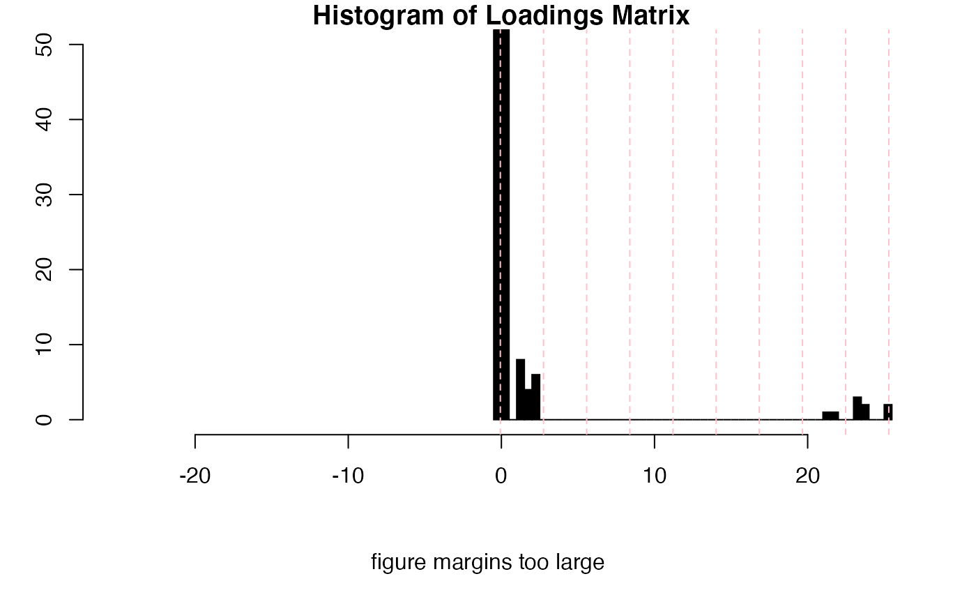
inspectLvls(res1,
  which = 11, ylim = c(0, 50),
  main = "Histogram of Loadings Matrix")