The Math Behind PCA
David T. Harvey1
Bryan A. Hanson2
2024-04-26
Source:vignettes/Vig_06_Math_Behind_PCA.Rmd
Vig_06_Math_Behind_PCA.RmdThis vignette is based upon LearnPCA version 0.3.4.
LearnPCA provides the following vignettes:
- Start Here
- A Conceptual Introduction to PCA
- Step By Step PCA
- Understanding Scores & Loadings
- Visualizing PCA in 3D
- The Math Behind PCA
- PCA Functions
- Notes
- To access the vignettes with
R, simply typebrowseVignettes("LearnPCA")to get a clickable list in a browser window.
Vignettes are available in both pdf (on CRAN) and html formats (at Github).
In this vignette we’ll look closely at how the data reduction step in PCA is actually done. This vignette is intended for those who really want to dig deep. It’s helpful if you know something about matrix manipulations, but we work hard to keep the level of the material accessible to those who are just learning.
Introduction
If you have read the Step By Step PCA vignette, you know that the first steps in PCA are:
- Center the data by subtracting the column means from the columns.
- Optionally, scale the data column-wise.
- Carry out the reduction step, typically using
prcomp.
For a data matrix with \(n\) rows of observations/samples and \(p\) variables/features, the results are the
- scores matrix with \(n\) rows and \(p\) columns, where each column corresponds to a principal component and the values are the scores, namely the positions of the samples in the new coordinate system.
- loadings matrix with \(p\) rows and \(p\) columns, which represent the contributions of each variable to each principal component.
In the Step By Step PCA vignette we also showed how to reconstruct or approximate the original data set by multiplying the scores by the transpose of the loadings.
In Figure 1 we show one way to represent the relationships between the original data matrix (\(\mathbf{X}\)), the loadings matrix (\(\mathbf{L}\)) and the scores matrix (\(\mathbf{S}\)).
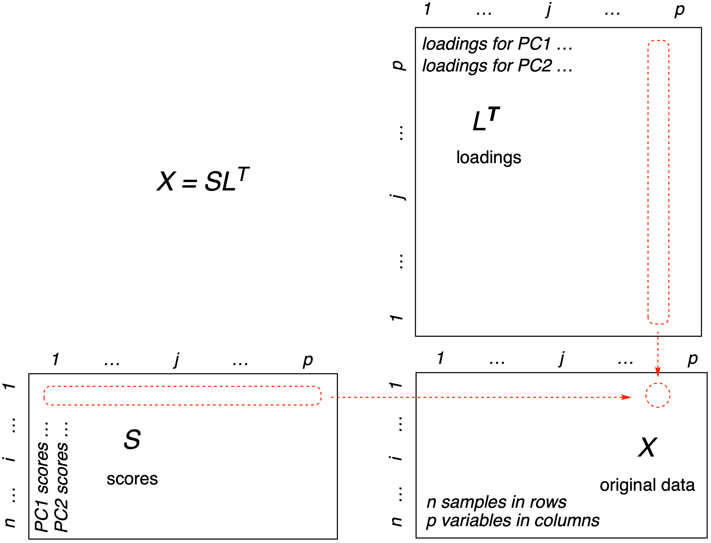
Figure 1: One way to look at the matrix algebra behind PCA. Reconstruction of the data matrix \(\mathbf{X}\) is achieved by multiplying the score matrix (\(\mathbf{S}\)) by the transpose of the loadings matrix (\(\mathbf{L^T}\)). The method of matrix multiplication is symbolized in the red-dotted outlines: Each element of row \(i\) of the scores matrix is multiplied by the corresponding element of column \(j\) of the transposed loadings. These results are summed to give a single entry in the original data matrix \(\mathbf{X}_{ij}\).
Figure 1 demonstrates that if we multiply the scores matrix (\(\mathbf{S}\)) by the transpose of the loadings matrix (\(\mathbf{L^T}\)), we get back the original data matrix (\(\mathbf{X}\)). When we start however, all we have is the original data matrix, how do we get the other two matrices? If we think of this as an algebra problem, we seem to be missing some variables; computing the loadings and scores matrices seems like it would be impossible, as there is not enough information. However, this is not a algebra problem, it is a linear algebra problem (linear algebra being the study of matrices). It is possible to determine the answer, even though we seem to be missing information, as we shall see shortly. The key is in something called matrix decompositions.3
Matrix Decompositions
In a moment we are going to look at two matrix decompositions in detail, the singular value decomposition (SVD) and the eigenvalue decomposition. These decompositions are representative of roughly a dozen matrix decompositions. A matrix decomposition or factorization breaks a matrix into pieces in such a way as to extract information and solve problems. The SVD is probably the most powerful decomposition there is – we will make extensive use of this insightful Twitter thread by Dr. Daniela Witten of the University of Washington. We also use this excellent Cross Validated answer by amoeba.
A short note however, before we dig deeper. Since we are using a computer to solve this problem, we need to keep in mind that using a computer is not quite the same as solving a problem using pencil and paper. On the computer, we usually have choices of algorithms to solve problems. Some algorithms are more robust than others. Algorithms need to take into account edge cases where the computation can become unstable. For instance, computers can only store numbers to a certain level of accuracy: when is “very small” actually zero in practice? We need to know this so we don’t try to divide by zero. This is only one example of problems that can arise when using a computer to calculate anything.
Finally, the two decompositions we are going to look at have something in common. Our approach will be to explain each without reference to the other, as this facilitates digestion and understanding of each (it doesn’t seem fair to require you to understand the 2nd one that you haven’t read while trying to understand the first one). Then, if you are still with us, we’ll look at what they have in common.
The SVD Decomposition
We’ll start from the original data matrix \(\mathbf{X}\) which has samples in rows and measured variables in columns. Let’s assume that we have column-centered the matrix. The SVD decomposition breaks this matrix \(\mathbf{X}\) into three matrices (dimensions in parentheses):4
\[\begin{equation} \tag{1} \mathbf{X}_{(n \ \times \ p)} = \mathbf{U}_{(n \ \times \ p)}\mathbf{D}_{(p \ \times \ p)}\mathbf{V}_{(p \ \times \ p)}^T \end{equation}\]
And here’s the equation without matrix dimensions. Remember that \(\mathbf{V}^T\) means “take the transpose” of \(\mathbf{V}\), interchanging rows and columns.
\[\begin{equation} \tag{2} \mathbf{X} = \mathbf{U}\mathbf{D}\mathbf{V}^T \end{equation}\]
The equation above is where we’d like to end up. How can we get there? Let’s start with What are these matrices?
- \(\mathbf{X}\) contains the original data.
- \(\mathbf{D}\) is a diagonal matrix, which means all non-diagonal elements are zero. The diagonal contains positive values sorted from largest to smallest. These are called the singular values.5
- The columns of \(\mathbf{V}\) are vectors giving the principal axes. These define the new coordinate system.
- The scores can be obtained by \(\mathbf{X}\mathbf{V}\) or \(\mathbf{U}\mathbf{D}\); scores are the projections of the data on the principal axes.
In addition, \(\mathbf{U}\) and \(\mathbf{V}\) are semi-orthogonal matrices,6 which means that when pre-multiplied by their transpose one gets the identity matrix:7
\[\begin{equation} \tag{3} \mathbf{U}^{T}\mathbf{U} = \mathbf{I} \end{equation}\]
\[\begin{equation} \tag{4} \mathbf{V}^{T}\mathbf{V} = \mathbf{I} \end{equation}\]
We’ll use this fact to great advantage when we implement a simple version of SVD in a moment.
First however, let’s use the two built-in functions svd and prcomp to compute the “accepted” answer for comparison to our simple implementation.
set.seed(30)
X <- matrix(rnorm(100*50), ncol = 50) # generate random data
X <- scale(X, center = TRUE, scale = FALSE) # always work with centered data
X_svd <- svd(X)
X_pca <- prcomp(X, center = FALSE) # already centered
A Simple Implementation of SVD
Now that we know what these matrices are, we can look into how to compute them. As mentioned earlier, the algorithm is everything here. As a simple example, we’ll look at an approach called “power iteration.” This is by no means the best approach, but it is simple enough that we can understand the idea. First, let’s generate some random data. In this simple example we are only going to compute the first principal component, so V is a vector, not a matrix (one can still do matrix multiplication with a vector, we just treat it as a “row vector” or a “column vector”).8 Note that the dimensions of the variables are chosen so that we can matrix multiply them (they are conformable matrices).
We’ll do a simple iterative calculation that computes the values of U and V. The loop runs for 50 iterations, and as it does the values of U and V are continuously updated and get closer to the actual answer.
V <- rnorm(50)
for (iter in 1:50) {
  U <- X %*% V # Step 1
  U <- U/sqrt(sum(U^2)) # Step 2
  V <- t(X) %*% U # Step 3
  V <- V/sqrt(sum(V^2)) # Step 4
 if ((iter %% 10) == 0L) { # report every 10 steps; print the correlation between
   cat("\nIteration", iter, "\n") # the current U or V and the actual values from SVD
   cat("\tcor with V:", sprintf("%f", cor(X_svd$v[,1], V)), "\n")
   cat("\tcor with U:", sprintf("%f", cor(X_svd$u[,1], U)), "\n")
   }
}
##
## Iteration 10
## cor with V: -0.931423
## cor with U: -0.917212
##
## Iteration 20
## cor with V: -0.998964
## cor with U: -0.998752
##
## Iteration 30
## cor with V: -0.999981
## cor with U: -0.999978
##
## Iteration 40
## cor with V: -1.000000
## cor with U: -0.999999
##
## Iteration 50
## cor with V: -1.000000
## cor with U: -1.000000Notice that there is no \(\mathbf{D}\) matrix in this calculation. This is because we are only calculating a single principal component, and therefore in this case \(\mathbf{D}\) is a scalar constant. We can drop it from the calculation. With that simplification, we can look at each step.
Step 1
The first step is to multiply the data matrix X by the initial estimate for V (remember at each iteration the estimate gets better and better). How does this relate to Equation (2)? If we drop \(\mathbf{D}\) from equation (2) we have:
\[\begin{equation} \tag{5} \mathbf{X} = \mathbf{U}\mathbf{V}^T \end{equation}\]
If we right multiply both sides by \(\mathbf{V}\) we have:
\[\begin{equation} \tag{6} \mathbf{X}\mathbf{V} = \mathbf{U}\mathbf{V}^T\mathbf{V} \end{equation}\]
which evaluates to:
\[\begin{equation} \tag{7} \mathbf{X}\mathbf{V} = \mathbf{U}\mathbf{I} = \mathbf{U} \end{equation}\]
because \(\mathbf{V}\) is a semi-orthogonal matrix. This is the line in the code.
Step 2
In this step we normalize (regularize, or scale) the estimate of U, by dividing by the square root of the sum of the squared values in U.9 This has the practical effect of keeping the values in U from becoming incredibly large and possibly overflowing memory.10
Step 3
Here we update our estimate of V. Similar to Step 1, we can rearrange Equation (2), this time by dropping \(\mathbf{D}\), pre-multiplying both sides by \(\mathbf{U}^T\) to give an identity matrix which drops out, and then transposing both sides:
\[\begin{equation} \tag{8} \mathbf{U}^T\mathbf{X} = \mathbf{U}^T\mathbf{U}\mathbf{V}^T \end{equation}\]
\[\begin{equation} \tag{9} \mathbf{U}^T\mathbf{X} = \mathbf{I}\mathbf{V}^T \end{equation}\]
\[\begin{equation} \tag{10} \mathbf{U}^T\mathbf{X} = \mathbf{V}^T \end{equation}\]
\[\begin{equation} \tag{11} (\mathbf{U}^T\mathbf{X})^T = (\mathbf{V}^T)^T \end{equation}\]
\[\begin{equation} \tag{12} \mathbf{X}^T\mathbf{U} = \mathbf{V} \end{equation}\]
which is the operation we see in the code snippet.11
Overall
Essentially what this algorithm is doing is alterating between the two calculations (for U, steps 1 & 2, then for V steps 3 & 4), with X constant. At each iteration these estimates improve, moving from the initial random value of V towards the best answer for both Vand U.
Reporting
You’ll notice that the code snippet above has a few lines to report the progress of the calculation. Every 10 steps the correlation between the current value of V with the official answer contained in X_svd$v is displayed (and the same for U). As you can see from the output the correlation is not bad after 10 iterations and only improves with more iterations. We report the correlation because the signs of the power iteration answers may vary from those computed by svd.12
Comparison to the Answer from svd
Let’s compare the absolute values of the two different answers:
## [1] 2.679147e-06## [1] 1.793972e-06As you can see, the values are essentially the same.
Comparison to the Answer from prcomp
We have seen that our estimate of U and V compared well to the results from the function svd. In practice users would probably use prcomp for PCA. So let’s compare to the results from prcomp.
## [1] 2.559261e-05## [1] 2.679147e-06In this case as well, the values compare favorably.
Notice that we have worked through the SVD without mentioning eigen-anything. That was one of our goals. Now let’s take a different point of view.
The Eigen Decomposition
The eigen decomposition is another way to decompose a data matrix. This decomposition breaks the data matrix \(\mathbf{X}\) into two matrices.13 Again, let’s assume \(\mathbf{X}\) has samples in rows, variables in columns, and has been centered.
\[\begin{equation} \tag{13} \mathbf{X}_{(n \ \times \ n)} = \mathbf{Q}_{(n \ \times \ n)}\mathbf{\Lambda}_{(n \ \times \ n)}\mathbf{Q}_{(n \ \times \ n)}^{T} \end{equation}\]
And here’s the equation without matrix dimensions.14
\[\begin{equation} \tag{14} \mathbf{X} = \mathbf{Q}\mathbf{\Lambda}\mathbf{Q}^{T} \end{equation}\]
The equation above is where we’d like to end up; it looks like a variation on the equation for SVD. How can we get there? Once again, let’s take inventory of the matrices in the equation.
- \(\mathbf{X}\) is the original data matrix. Notice the dimensions are \(n \times n\), unlike in SVD. In other words, it is a square matrix. Your data is not square you say? Eigen decomposition requires an square matrix. Fortunately, there’s a simple fix for this. We can work instead with the covariance matrix, which is square: \(\mathbf{X}^T\mathbf{X}/(n - 1)\). This retains all the structure of the original data.15
- \(\mathbf{Q}\) is square matrix that whose columns will contain the eigenvectors. \(\mathbf{Q}\) is also an orthogonal matrix (discussed earlier in the SVD section). Notice that \(\mathbf{Q}\) appears twice in (14), the second time as its transpose.
- \(\mathbf{\Lambda}\) (upper case Greek letter Lambda) is a diagonal matrix, very similar in purpose to \(\mathbf{D}\) in SVD. All non-diagonal elements are zero. The diagonal contains values sorted from largest to smallest. These are called the eigenvalues.
So what are eigenvectors and eigenvalues? The eigenvalues are related to the amount of variance explained for each principal component. The eigenvectors are the principal axes, which as we have seen constitute a new coordinate system for looking at the data (see the Visualizing PCA in 3D vignette for details). If we post-multiply the original data by the eigenvectors in \(\mathbf{Q}\) we get the scores:
\[\begin{equation} \tag{15} \mathbf{X}\mathbf{Q} = scores \end{equation}\]
And the loadings are simply the eigenvectors in \(\mathbf{Q}\).
A Simple Implementation of the Eigen Decomposition
As we did for SVD, we can use a power iteration to compute estimates for the first eigenvector.
Next, we’ll use the built-in function eigen to compute the “official” answer for comparison to our results.
A simple iterative process as we did for SVD will continuously update the value of Q.
Q <- rnorm(50)
for (iter in 1:50) {
  Q <- X_cor %*% Q # Step 1
  Q <- Q/sqrt(sum(Q^2)) # Step 2

 if ((iter %% 5) == 0L) { # report every 5 steps; print the correlation between
   cat("\nIteration", iter, "\n") # the current Q and the actual values from SVD
   cat("\tcor with Q:", sprintf("%f", cor(X_eig$vectors[,1], Q)), "\n")
   }
}
##
## Iteration 5
## cor with Q: -0.551169
##
## Iteration 10
## cor with Q: -0.848349
##
## Iteration 15
## cor with Q: -0.963039
##
## Iteration 20
## cor with Q: -0.991606
##
## Iteration 25
## cor with Q: -0.998081
##
## Iteration 30
## cor with Q: -0.999555
##
## Iteration 35
## cor with Q: -0.999896
##
## Iteration 40
## cor with Q: -0.999975
##
## Iteration 45
## cor with Q: -0.999994
##
## Iteration 50
## cor with Q: -0.999999How does the final estimate for Q compare to the official answer? We can check our result as before:
## [1] -3.010147e-05Good work by the power iteration!
The Relationship Between SVD and Eigen Decomposition
It’s apparent that SVD and the eigen decomposition have a lot in common. The R function prcomp uses the svd function “under the hood”, and the function princomp uses eigen under the hood. The vignette PCA Functions goes into greater detail about the similarities and differences between these two decompositions as implemented in R.
Singular Values vs Eigenvalues
We’ve talked about “values” in the context of each decomposition. Is this terminology accidental, or is there a relationship? If you square the singular values from SVD and divide by \(n -1\), you get the eigenvalues. Here “diagonal” means take the diagonal elements of the matrix (which would be a vector of values):
\[\begin{equation} \tag{16} (diagonal(\mathbf{D}))^2/(n - 1) = diagonal(\mathbf{\Lambda}) \end{equation}\]
Either of these “values” can be used to compute the amount of variance explained by each principal component. Details are in the PCA Functions vignette.
A Note About the Meaning of “loadings”
Before going further, we need to make something clear. In R, the loadings reported by prcomp are actually the eigenvectors of the covariance matrix of the original data matrix (discussed here and here). This is very clear in the help file for prcomp, and from the code checking the results above. However, this is not a universally accepted definition; R is actually a bit of an outlier. A more generally accepted definition for loadings is given below, where N is the number of samples. This use of the term loadings is sometimes referred to as “standardized loadings”.
\[\begin{equation} \tag{17} \mathbf{L} = \mathbf{V}\frac{\mathbf{D}}{\sqrt{N-1}} \end{equation}\]
The important thing here is that the definition above is just a scaled version of the value that R returns. Figure 2 is a comparison of the first column of each use of the term “loadings”.
R_loadings <- X_pca$rotation[,1]
std_loadings <- (X_svd$v %*% diag(X_svd$d)/(nrow(X - 1)))[,1]
plot(R_loadings, std_loadings, xlab = "R's notion of loadings", ylab = "Standard notion of loadings")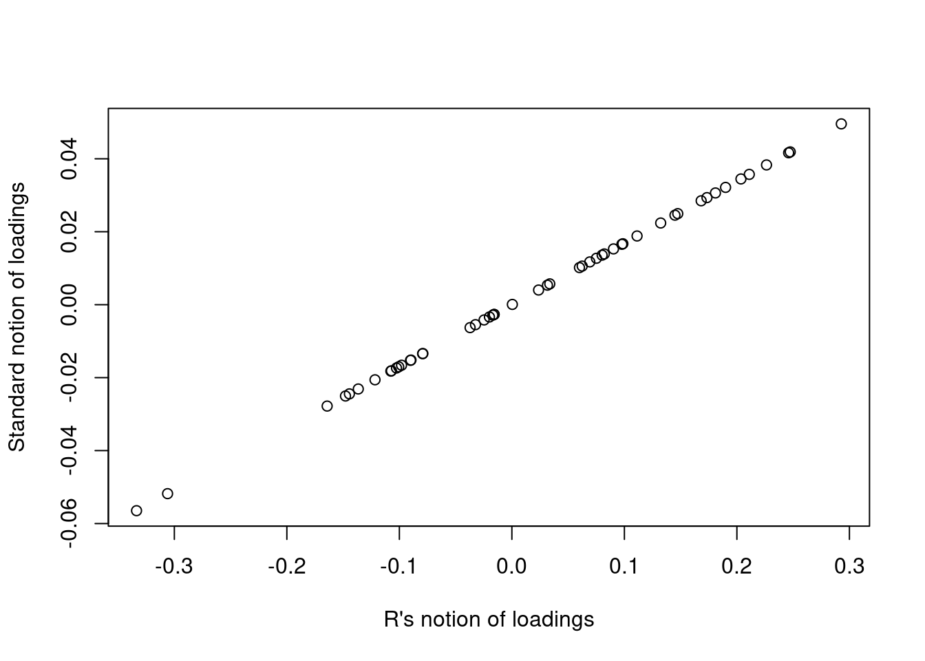
Figure 2: A comparison of the notion of loadings as delivered by R and a more standard definition.
This means that the usual verbal interpretation of loadings, namely that they express the relative contribution of each variable to the scores, is valid using either notion.
Algorithmic Reality
The two simple implementations described above are very limited. They are in no way suitable for use with real data, but they do serve as a conceptual introduction. In reality, carrying out PCA on real data sets in a robust manner requires rather complex algorithms, well beyond the scope of these documents. If you want a brief taste, the Wikipedia article and this StackOverflow answer may satisfy your needs. A more intermediate discussion can be found in Chapter 3 “Principal Components Analysis” in Varmuza and Filzmoser (2009).
The NIPALS Algorithm
In addition to SVD and Eigen decomposition, there is another algorithm we should discuss. NIPALS stands for Non-linear Iterative PArtial Least Squares. NIPALS is a very important algorithm because:
- One can limit the number of principal components one calculates, you don’t have to calculate all of them as you do with SVD and the Eigen decomposition. If you have a very large data set, calculating a limited number of principal components and save time and reduce memory use.
- Missing values are acceptable, unlike the two decompositions discussed earlier.
NIPALS is not so much another decomposition but rather more a direct attack on the equation featured in Figure 1:
\[\begin{equation} \tag{18} \mathbf{X} = \mathbf{S} \mathbf{L^T} \end{equation}\]
A Simple Implementation of NIPALS
Here is a function that will compute PCA using the NIPALS algorithm. The key math steps here are just rearrangements of (18).
simpleNIPALS <- function(X, pcs = 3, tol = 1e-6) {
  S <- NULL # a place to store the scores
  L <- NULL # a place to store the loadings
  for (pc in 1:pcs) { # compute one PC at a time
    s_old <- X[,1] # initial estimate of the score Note 1
    done <- FALSE # flag to track progress
    while (!done) { # Note 2
      l <- t(X) %*% s_old # compute/improve/update loadings estimate
      l <- l/sqrt(sum(l^2)) # scale by l2 norm
      s_new <-X %*% l # compute/improve/update scores estimate
      err <- sqrt(sum((s_new - s_old)^2)) # compute the error of the score estimate
      if (err < tol) {done <- TRUE; next} # check error against tolerance,
                                          # exit if good
      s_old <- s_new # if continuing, use the improved score estimate
                     # next time through while loop
    }
    X <- X - s_new %*% t(l) # "deflate" the data by removing the
                            # contribution of the results so far Note 3
    S <- cbind(S, s_new) # add the most recent scores to the growing results
    L <- cbind(L, l) # add the most recent loadings to the growing results
  }
  list(Scores = S, Loadings = L) # return the answers
}
If you looked carefully at our earlier simple implementations of SVD and eigen decomposition, you probably noticed that this simple NIPALS function is also using power iteration and is very similar. Let’s draw attention to a few things:
- Note 1: Here we select the first column of \(\mathbf{X}\) as our initial estimate of the scores. In our simple implementations of SVD and eigen decomposition we used a random draw to determine the initial estimate.
-
Note 2: All the work is done inside this
whileloop, which runs until the error is below the tolerance. The basic flow is to start with the initial estimate, update scores and loadings, then then feed these back in as better estimates. This is exactly the concept used in the other implementation, we are just doing it until the tolerance is reached, rather than running it a fixed number of iterations. - Note 3: This “deflation” step is unique to NIPALS. Once we have estimates for the scores with minimal error, we reconstruct the original data following equation (18), and subtract this from the original \(\mathbf{X}\) to give a “deflated” \(\mathbf{X}\) which is then processed as before if we have more PCs to compute.
Checking Our work
Let’s run this function and compare to the previous accepted answers.
## [1] 4.482769e-08## [1] 5.605989e-09## [1] 4.482769e-08## [1] 5.605989e-09These are satisfying results that show our simple NIPALS function gives good results.
Tying Things Together
In our simple implementation of SVD and eigen decomposition, we used power iteration because it was fairly easy to relate to the fundamental equations ((1) and (14)). As we mentioned above however, power iteration is not the best way to actually do either SVD or eigen decomposition. However, power iteration is the method used in NIPALS, so our time was well spent to understand the principle.
Works Consulted
In addition to references and links in this document, please see the Works Consulted section of the Start Here vignette for general background.
References
Professor of Chemistry & Biochemistry, DePauw University, Greencastle IN USA., harvey@depauw.edu↩︎
Professor Emeritus of Chemistry & Biochemistry, DePauw University, Greencastle IN USA., hanson@depauw.edu↩︎
If you need an introduction to linear algebra, there are many good books, but we particularly recommend Singh (2014) or Savov (2020).↩︎
The singular values are used to calculate the variance explained by each principal component. We’ll have more to say about that later.↩︎
For semi-orthogonal matrices (or orthogonal matrices for that matter), \(A^TA = AA^T = I\). Semi-orthogonal matrices are rectangular. For non-rectangular orthogonal matrices, if \(n > p\), the dot product of any column with itself is 1, and the dot product of any column with a different column is zero. If \(n < p\), then it is the rows rather than the columns that are relevant. See the Wikipedia article.↩︎
The identity matrix \(\mathbf{I}\) is a square matrix with ones on the diagonal and zeros everywhere else. The identity matrix can pre- or post-multiply any other matrix and not affect that matrix.↩︎
When refering to the mathematical equations, we’ll use \(\mathbf{X}\), but when referencing the values we compute, we’ll use
X.↩︎This is the \(L^2\) or Euclidean norm, generally interpreted as a length. It can also be computed as \(U^TU\).↩︎
As the values grow larger and larger, first we lose precision and eventually the numbers become too big to store.↩︎
The operation from equation (11) to (12) is based upon the following property in linear algebra: \((AB)^T\) = \(B^TA^T\).↩︎
From
?prcomp“The signs of the columns of the rotation matrix are arbitrary, and so may differ between different programs for PCA, and even between different builds of R.” From?princomp“The signs of the columns of the loadings and scores are arbitrary, and so may differ between different programs for PCA, and even between different builds of R: fix_sign = TRUE alleviates that.” We discuss the origin of the different signs in more detail in PCA Functions vignette.↩︎Eigenvalues and eigenvectors are extremely important in linear algebra. The concept is usually introduced in the simpler form \(Au = \lambda u\).↩︎
One also sees this written \(\mathbf{X} = \mathbf{Q}\mathbf{\Lambda}\mathbf{Q}^{-1}\). This is equivalent because for orthogonal matrices \(\mathbf{A}^T = \mathbf{A}^{-1}\).↩︎
We can also use the correlation matrix, which is evaluated via the same formula. For covariance, one centers the raw data columns. For correlation, one centers the raw data and then scales them by their standard deviation.↩︎