A Comparison of Functions for PCA
David T. Harvey1
Bryan A. Hanson2
2024-04-26
Source:vignettes/Vig_07_Functions_PCA.Rmd
Vig_07_Functions_PCA.RmdThis vignette is based upon LearnPCA version 0.3.4.
LearnPCA provides the following vignettes:
- Start Here
- A Conceptual Introduction to PCA
- Step By Step PCA
- Understanding Scores & Loadings
- Visualizing PCA in 3D
- The Math Behind PCA
- PCA Functions
- Notes
- To access the vignettes with
R, simply typebrowseVignettes("LearnPCA")to get a clickable list in a browser window.
Vignettes are available in both pdf (on CRAN) and html formats (at Github).
There are four base functions in R that can carry out PCA analysis.3 In this vignette we will look at each of these functions and how they differ.
prcomp
prcomp is probably the function most people will use for PCA, as it will handle input data sets of arbitrary dimensions (meaning, the number of observations \(n\) may be greater or less than the number of measured variables, \(p\)). prcomp can do centering or scaling for you, but it also recognizes when the data passed to it has been previously centered or scaled via the scale function.4 Internally, prcomp is a wrapper for the svd function (which we’ll discuss below). This means that prcomp uses svd “under the hood” and repackages the results from svd in a more useful form.
princomp
In contrast to prcomp, princomp cannot directly handle the situation where \(p > n\), so it is not as flexible. In addition, princomp uses function eigen under the hood, and eigen only accepts square matrices as input (where \(n = p\)). However, princomp will accept a rectangular matrix with \(n > p\) because internally princomp will convert the input matrix to either the covariance or correlation matrix before passing the new matrix to eigen (the choice depends upon the arguments). Both the covariance and correlation matrices are square matrices that eigen can process. As we shall see below, they give the same scores as the raw data (as long as the scaling is consistent).
Covariance
Let’s take quick look at covariance and correlation. First, we’ll create some data to play with:
## [1] 4 5If you center the columns of \(A\), take \(A^TA\) and then divide by \(n -1\) you get the covariance matrix. We can verify this via the built-in function cov. Covariance describes how the variables track each other. Covariance is unbounded, which means its values can range over \(\pm \infty\).
Ac <- scale(A, center = TRUE, scale = FALSE)
covA <- (t(Ac) %*% Ac)/(nrow(Ac) -1)
dim(covA) # it's square
## [1] 5 5## [1] TRUECorrelation
If instead you center the columns of \(A\), i.e. scale the columns by dividing by their standard deviations, take \(A^TA\) and then divide by \(n -1\) you get the correlation matrix. Like covariance, correlation describes how the variables track each other. However, correlation is bounded on \([-1, 1]\). In effect, correlation is covariance normalized to a constant scale. Again we can verify this with the built-in function cor:
Acs <- scale(A, center = TRUE, scale = TRUE)
corA <- (t(Acs) %*% Acs)/(nrow(Acs) -1)
dim(corA) # square like covA
## [1] 5 5## [1] TRUEImportantly, the covariance and correlation matrices contain the same information about the relationship of the original variables, so that PCA of either of these matrices or the original data matrix will give the same results. This will be demonstrated in the next section.
prcomp vs princomp
Let’s compare the results from each function. Let’s use a portion of the mtcars data set that is small enough that we can directly print and inspect the results. Converting to a matrix is not necessary but saves some typing later.
Next we’ll calculate PCA using both functions. Note that the arguments for prcomp will center and autoscale the data before doing the key computation. For princomp, the data will be centered and the correlation matrix computed and analyzed.5
Compare the Scores
We can directly examine the results for the scores:
pca$x## PC1 PC2 PC3 PC4 PC5
## Mazda RX4 -1.0479560 0.02812191 0.20417776 -0.23574115 0.19041257
## Datsun 710 -1.9187384 0.62012252 0.03701878 0.18764497 -0.22980986
## Hornet Sportabout 1.2408888 -0.34050957 0.42754323 0.36253075 0.14423806
## Duster 360 2.0345815 -0.21095796 -0.13943434 -0.29895647 -0.47011484
## Merc 230 -1.8534734 0.48404256 -0.14340048 0.26855557 -0.16691142
## Merc 280C -0.6943891 0.26998531 -0.09844637 -0.54336861 0.22228448
## Merc 450SL 1.1825263 0.02862923 0.67289539 -0.07586040 -0.04125809
## Cadillac Fleetwood 2.6175010 0.33221478 -0.40782360 0.17057754 0.39558239
## Chrysler Imperial 2.1330076 -0.38158713 -0.35443033 0.11037449 -0.13208565
## Honda Civic -3.6939483 -0.83006166 -0.19810003 0.05424331 0.08766235
prin$scores## Comp.1 Comp.2 Comp.3 Comp.4 Comp.5
## Mazda RX4 1.1046426 -0.02964310 0.21522225 -0.24849299 -0.20071247
## Datsun 710 2.0225279 -0.65366653 0.03902122 0.19779517 0.24224086
## Hornet Sportabout -1.3080117 0.35892860 0.45067014 0.38214097 -0.15204026
## Duster 360 -2.1446372 0.22236922 -0.14697670 -0.31512779 0.49554455
## Merc 230 1.9537325 -0.51022565 -0.15115738 0.28308243 0.17594008
## Merc 280C 0.7319504 -0.28458951 -0.10377159 -0.57276081 -0.23430841
## Merc 450SL -1.2464922 -0.03017786 0.70929402 -0.07996388 0.04348984
## Cadillac Fleetwood -2.7590883 -0.35018513 -0.42988382 0.17980451 -0.41698045
## Chrysler Imperial -2.2483874 0.40222815 -0.37360237 0.11634493 0.13923050
## Honda Civic 3.8937634 0.87496181 -0.20881577 0.05717747 -0.09240423Notice that the absolute values of the scores are similar, but not identical. This is because different algorithms were used in each case. Notice too that the pattern of positive and negative values is complex, it’s not as if one is simply the negative of the other. We’ll have more to say about this momentarily.
## [1] "Mean relative difference: 0.0513167"Another way to compare these results is to overlay a plot of the scores from each method. Figure 1 shows the results. The pattern of positive and negative scores becomes much clearer in this plot.
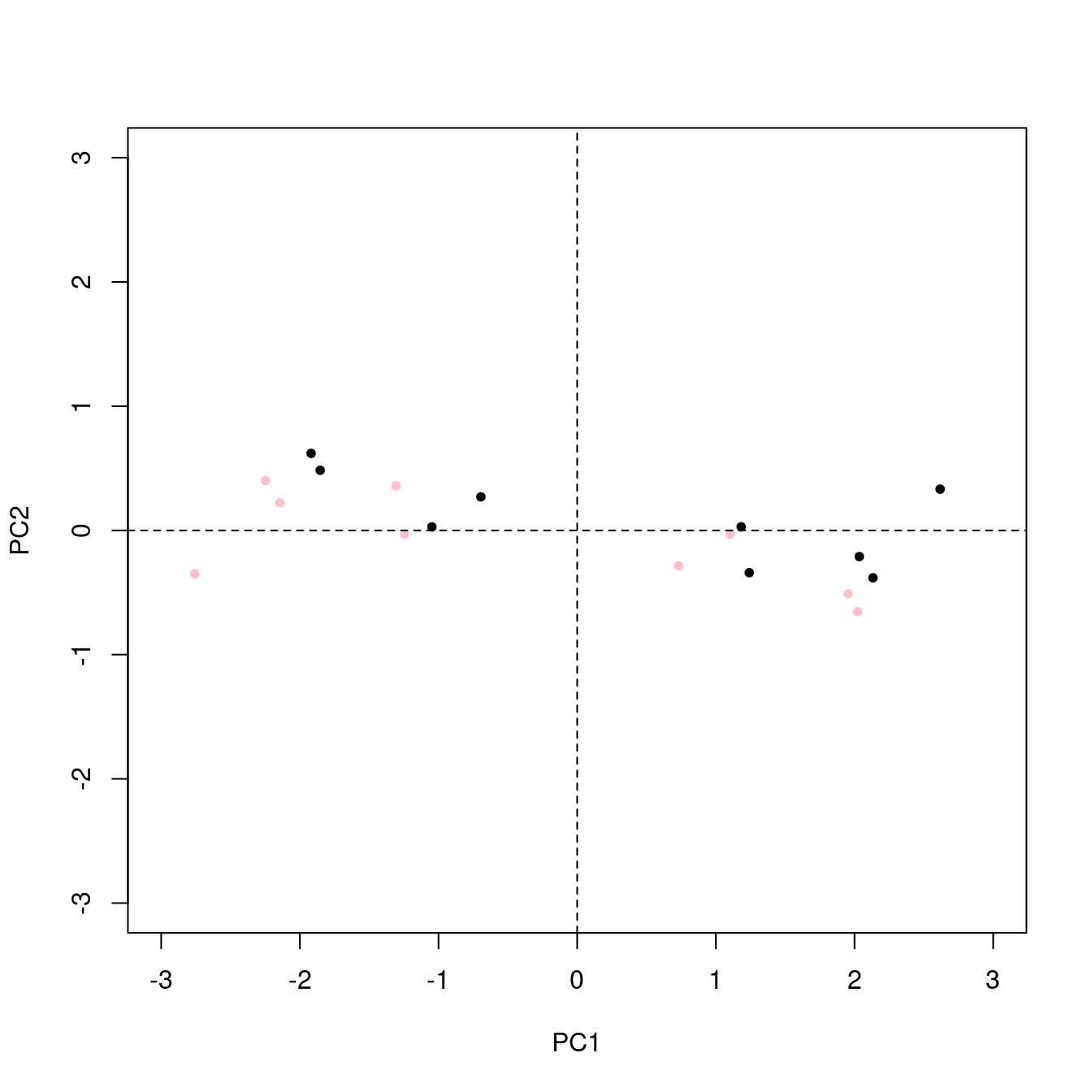
Figure 1: Comparison of scores computed by prcomp (black points) and princomp (pink points). Note that they are related by a 180 degreee rotation about an axis out of paper at the origin (plus a little wiggle due to algorithm differences).
Compare The Loadings
Let’s do the same for the loadings. For the princomp results we have to extract the loadings because they are stored in an usual form by today’s practices.
pca$rotation## PC1 PC2 PC3 PC4 PC5
## mpg -0.4436384 -0.5668868 0.3843013 0.4943128 -0.2996526
## cyl 0.4445134 -0.5119978 0.5168597 -0.3609456 0.3779423
## disp 0.4496206 -0.3071229 -0.4852451 0.6128739 0.3040389
## hp 0.4545077 -0.2474375 -0.1952584 -0.2123927 -0.8055811
## drat -0.4436856 -0.5108305 -0.5581934 -0.4523805 0.1611437
prin_loads <- matrix(prin$loadings, ncol = 5, byrow = FALSE)
prin_loads
## [,1] [,2] [,3] [,4] [,5]
## [1,] 0.4436384 0.5668868 0.3843013 0.4943128 0.2996526
## [2,] -0.4445134 0.5119978 0.5168597 -0.3609456 -0.3779423
## [3,] -0.4496206 0.3071229 -0.4852451 0.6128739 -0.3040389
## [4,] -0.4545077 0.2474375 -0.1952584 -0.2123927 0.8055811
## [5,] 0.4436856 0.5108305 -0.5581934 -0.4523805 -0.1611437## [1] TRUEThe absolute value of the loadings from each method are identical, while the actual pattern of positive and negative values is complex as we saw for the scores. Why is this? Recall from the Understanding Scores and Loadings vignette that the loadings are the cosines of the angles through which the original axes are rotated to get to the new coordinate system. As cosine is a periodic function, if one rotates the reference frame 30 degrees to line up with the data better, the same alignment can also be achieved by rotating 30 + 180 degrees or 30 - 180 degrees. However, the latter two operations will give the opposite sign for the cosine value. This is the origin of the pattern of signs in the loadings; essentially there are positive and negative cosine values that both describe the needed reorientation equally well. Once the sign of the first value is chosen, the signs of the other values are meaningful only in that context.
As for the scores, a visual comparison of the results from each method will help us understand the relationship. In this case, we’ll just look at the signs of the loadings, and we’ll display the loadings for PC1 followed by the loadings for PC2 etc. Figure 2 makes clear that the two methods return loadings which sometimes have the same sign, and sometimes the opposite sign.
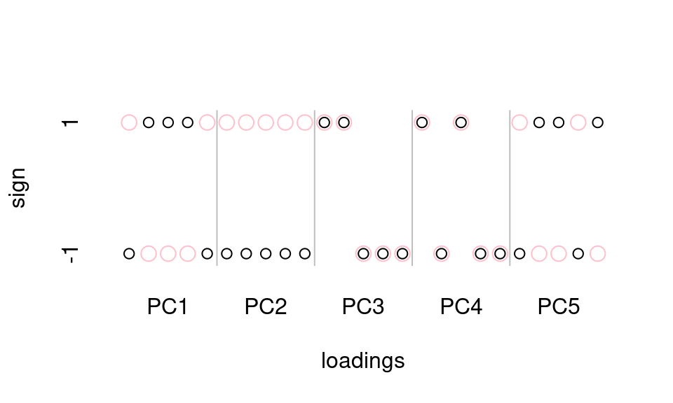
Figure 2: A comparison of the signs of the first loadings from prcomp (black circles) and princomp (pink circles). Where the circles coincide, the value of the loading from each method is the same.
The key takeaway here is that regardless of the signs of the scores and the loadings, the results from a particular function are internally consistent.
Compare the Variance Explained
For completeness, let’s make sure that each method returns the same variance explained values.
summary(pca)## Importance of components:
## PC1 PC2 PC3 PC4 PC5
## Standard deviation 2.1297 0.44706 0.34311 0.2846 0.25636
## Proportion of Variance 0.9071 0.03997 0.02354 0.0162 0.01314
## Cumulative Proportion 0.9071 0.94711 0.97066 0.9869 1.00000
summary(prin)## Importance of components:
## Comp.1 Comp.2 Comp.3 Comp.4 Comp.5
## Standard deviation 2.1297181 0.44706195 0.34311033 0.28459249 0.2563571
## Proportion of Variance 0.9071398 0.03997288 0.02354494 0.01619858 0.0131438
## Cumulative Proportion 0.9071398 0.94711269 0.97065763 0.98685620 1.0000000Clearly the numerical results are the same. You can see that the labeling of the results is different between the two functions. These labels are internally stored attributes. In the several places below we’ll ignore those labels and just check that the numerical output is the same.
Reconstruct the Original Data
While the pattern of positive and negative scores and loadings differs between algorithms, in any particular case the signs of the loadings and scores work together properly. We can use the function PCAtoXhat from this package to reconstruct the original data, and compare it to the known original data. This function recognizes the results from either prcomp or princomp and reconstructs the original data, accounting for any scaling and centering.
MTpca <- PCAtoXhat(pca) # not checking attributes as the internal labeling varies between functions
all.equal(MTpca, mt, check.attributes = FALSE)
## [1] TRUE## [1] TRUEAs you can see each function is reconstructing the data faithfully. And in the process we have shown that one gets the same results starting from either the centered and scaled original matrix, or the matrix which has been centered, scaled and then converted to its correlation matrix. Hence either approach extracts the same information, proving that the correlation matrix contains the same relationships that are present in the raw data.6
svd
As stated earlier, prcomp uses svd under the hood. Therefore we should be able to show that either function gives the same results. The key difference is that svd is “bare bones” and we have to prepare the data ourselves, and reconstruct the data ourselves. Let’s go.
First, we’ll center and scale the data, because svd doesn’t provide such conveniences.
mt_cen_scl <- scale(mt, center = TRUE, scale = TRUE)Then conduct svd:
sing <- svd(mt_cen_scl)Compare to the Scores from prcomp
The math behind extracting the scores and loadings is discussed more fully in the Math Behind PCA vignette. Here we use the results shown there to compare scores and loadings.
## [1] TRUECompare to the Loadings from prcomp
all.equal(sing$v, pca$rotation, check.attributes = FALSE)## [1] TRUE
eigen
princomp uses eigen under the hood, and so we should be able to show that these functions give the same results. Like svd, eigen is “bare bones” so we’ll start from the centered and scaled data set. In this case however, we also need to compute the correlation matrix, something that princomp did for us, but eigen expects you to provide a square matrix (either raw data that happens to be square, but more likely the covariance or correlation matrix).
Wrap Up
Table 1 summarizes much of what we covered above.
| prcomp | svd | princomp | eigen | |
|---|---|---|---|---|
| algorithm | uses svd | svd | uses eigen | eigen |
| input dimensions | \(n \times p\) | \(n \times p\) | \(n \times p\) | \(n \times n\) |
| user pre-processing | center; scale | center; scale | don’t do it! | center; scale; cov or cor |
| internal pre-processing | center; scale | none | center; cov or cor | none |
| call | \(pca \leftarrow prcomp(X)\) | \(sing \leftarrow svd(X)\) | \(prin \leftarrow princomp(X)\) | \(eig \leftarrow eigen(X)\) |
| scores | \(pca\$x\) | \(X \times sing\$v\) | \(prin\$scores\) | \(X \times eig\$vectors\) |
| loadings | \(pca\$rotation\) | \(sing\$v\) | \(prin\$loadings\) | \(eig\$vectors\) |
| pct variance explained | \(\cfrac{100*pca\$sdev^2}{sum(pca\$sdev^2)}\) | \(\cfrac{100*sing\$d^2}{sum(sing\$d^2)}\) | \(\cfrac{100*prin\$sdev^2}{sum(prin\$sdev^2)}\) | \(\cfrac{100*eig\$values}{sum(eig\$values)}\) |
Works Consulted
In addition to references and links in this document, please see the Works Consulted section of the Start Here vignette for general background.
Professor of Chemistry & Biochemistry, DePauw University, Greencastle IN USA., harvey@depauw.edu↩︎
Professor Emeritus of Chemistry & Biochemistry, DePauw University, Greencastle IN USA., hanson@depauw.edu↩︎
And there are numerous functions in user-contributed packages that “wrap” or implement these base functions in particular contexts.↩︎
This works because the
scalefunction adds attributes to its results, andprcompchecks for these attributes and uses them if present.↩︎In
princompthere is no argument regarding centering. The documentation is silent on this. However, if you look at the source code (viastats:::princomp.default) you discover that it callscov.wtwhich indeed centers, and gives the covariance matrix unless you set the argumentcor = TRUEin which case you get the correlation matrix.↩︎Proof that the covariance matrix gives the same results is left as an exercise!↩︎